Information Geometry: When Probability Distributions Become Points

We usually imagine a point as something like $(x,y)$ . Information geometry asks us to entertain a stranger possibility:

What if each point is an entire probability distribution?

Consider the family of normal distributions

\mathcal N(\mu,\sigma^2).

Every pair $(\mu,\sigma)$ identifies one distribution, so the family itself forms a two-dimensional parameter space.

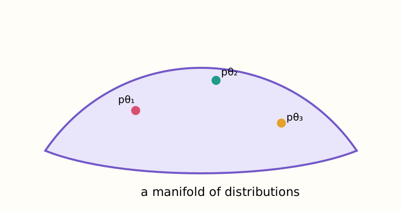
Curved parameter surface whose points represent probability distributions. — Each point represents a complete distribution. Moving on the surface means changing the distribution.

But what should distance mean?

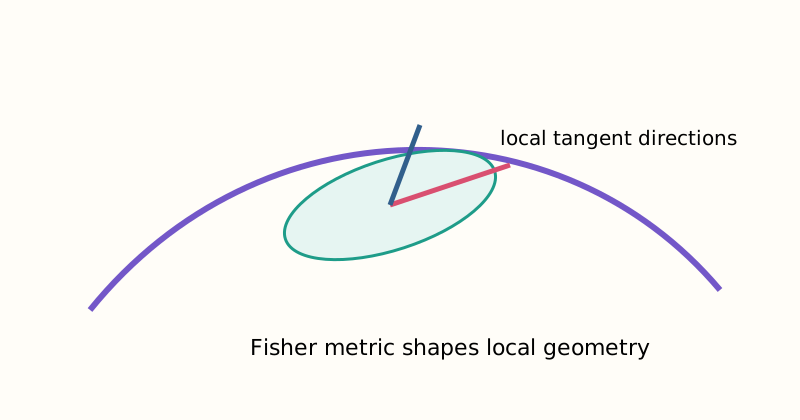
Ordinary Euclidean distance between parameter vectors depends on how we choose the parameters. Information geometry instead derives a local metric from the statistical model itself: the Fisher information.

For parameters $\theta$ ,

I(\theta) = \mathbb E_\theta \left[ \nabla_\theta\log p(X\mid\theta) \nabla_\theta\log p(X\mid\theta)^\top \right].

This acts like a position-dependent inner product on tangent directions.

Two local tangent directions on a curved statistical manifold with ellipses representing local metric geometry. — The Fisher metric tells us which tiny changes in parameters are statistically distinguishable.

KL divergence is nearby—but not a distance

The Kullback–Leibler divergence

D_{\mathrm{KL}}(p\|q) = \mathbb E_p\left[\log\frac{p(X)}{q(X)}\right]

is asymmetric, so it is not a metric. Yet its local second-order behavior is intimately related to Fisher information.

That is the doorway into a beautiful subject where probability, differential geometry, statistics and machine learning meet.